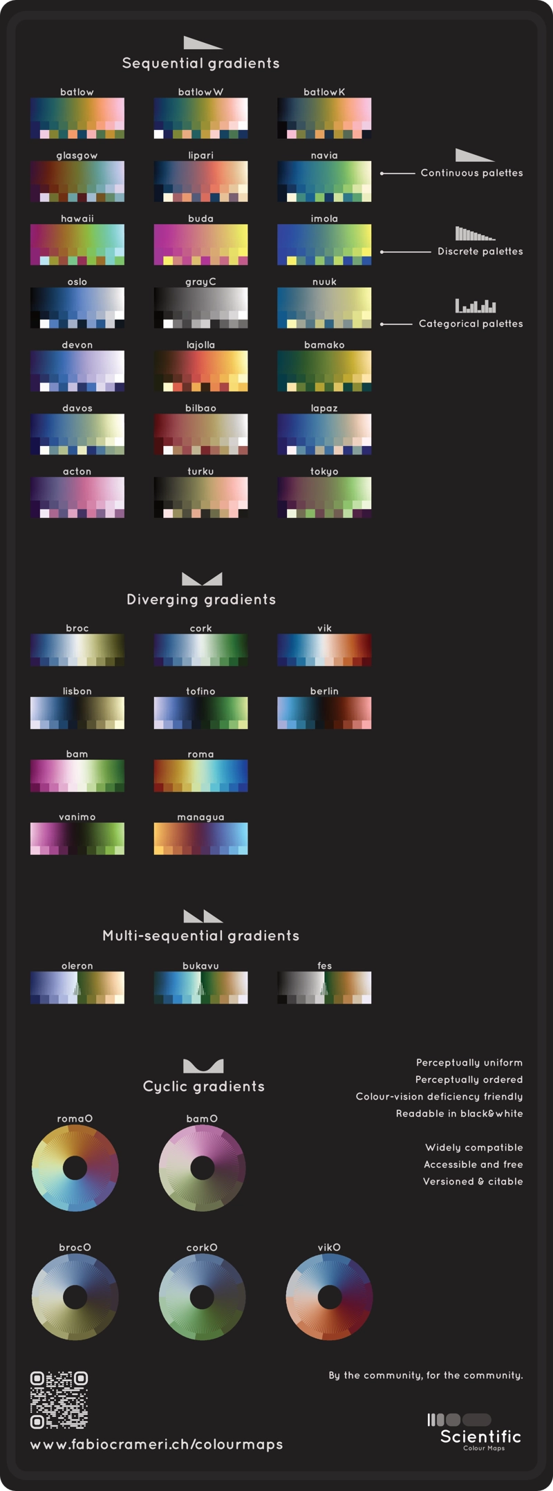
Fairly representing data
The colour gradients are perceptually uniform and ordered to represent data both fairly – without visual distortion – and intuitively

Accurate data visualisation needs
accurate scales readable by everyone.
#UseBatlow
The colour gradients are perceptually uniform and ordered to represent data both fairly – without visual distortion – and intuitively
The colour combinations are readable both by colour-vision deficient and colour-blind people, and even when printed in black&white
The colour maps and their diagnostics are permanently archived and versioned to enable upgrades and acknowledge developers and contributors
Crameri, F. (2018). Scientific colour maps. Zenodo. https://doi.org/10.5281/zenodo.1243862
Crameri, F. (2018), Geodynamic diagnostics, scientific visualisation and StagLab 3.0, Geosci. Model Dev., 11, 2541-2562, https://doi.org/10.5194/gmd-11-2541-2018
Crameri, F., G.E. Shephard, and P.J. Heron (2020), The misuse of colour in science communication, Nature Communications, 11, 5444, https://doi.org/10.1038/s41467-020-19160-7

MatLab, Python, Julia, R, GMT, QGIS, Ncview, Ferret, Plotly, Paraview, VisIt, Mathematica, Gnuplot, Surfer, d3, SKUA-GOCAD, Petrel, XMapTools, COMSOL Multiphysics, Fledermaus, Qimera, ImageJ, Fiji, Kingdom, Originlab, GIMP, Inkscape, Adobe Photoshop, and more...
➡ Extra formats for QPS software
➡ Extra formats for Kingdom software
➡ Extra formats for Originlab software
➡ Extra formats for Adobe Photoshop
➡ Extra formats for Adobe Illustrator
➡ Extra formats for OpendTect software
➡ Convenience package for GPlates
StagLab 3.0 and later
GMT 6.0 and later
TopoToolbox 2.2 and later
Geoscience ANALYST 2.80 and later
Igor Pro 9.0 and later
XMapTools 3.4.1 and later
KDE LabPlot 2.9 and later
Gen3sis 1.5 and later
SeisLib 0.5.1 and later
iolite 4.8.7 and later
Inclusivity: Apple macOS application including a colour scheme editor and accessibility tester to develop WCAG-proof iOS and macOS apps.
The design of batlow
The design of cyclic Scientific colour maps
The design of categorical Scientific colour maps
Colour use
Learn the do's and don'ts of using colour as an information carrier for scientifically-accurate and universally-inclusive data representation.
Figure design
Learn about the key principles and tools of graphic design and a recipe to make good science graphics.
Presentation design
Learn how to easily create effective presentations (Talks, PICOs, Posters, Online displays) of complicated topics.